Example

An overview of the package functionality is illustrated with the following example. Let

\[ f(\boldsymbol{x}) = \boldsymbol{x}'\boldsymbol{A}\boldsymbol{x} - 2\boldsymbol{b}'\boldsymbol{x} \]

denote a quadratic objective function in \(\boldsymbol{x}\), which is in the \(d\)-dimensional real space. If \(\boldsymbol{A}\) is a positive-definite \(d\times d\) matrix, then the unique minimum of \(f(\boldsymbol{x})\) is \(\boldsymbol{x}_{opt} = \boldsymbol{A}^{-1}\boldsymbol{b}\).

For example, suppose we have

import numpy as np

A = np.array([[3., 2.],
              [2., 7.]])
b = np.array([1., 10.])

Then we have that the optimal solution is \(\boldsymbol{x}_{opt} = (-0.765, 1.647)\). Now, projplot allows us to complete a visual check. The following information will need to be provided:

• The objective function (obj_fun): This can be either a vectorized or non-vectorized function.

• Optimal values (x_opt): This will be the optimal solution for your function.

• Upper and lower bounds for each parameter (x_lims): This will provide an initial range of values to observe.

• Parameter names (x_names): These are the names of your parameters in the plots.

• The number of points to plot for each parameter (n_pts): This is the number of points that each parameter will be evaluated at for their respective plot.

Setup

# Optimal values
x_opt = np.array([-0.765,  1.647])

# Upper and lower bounds for each component of x
x_lims = np.array([[-3., 1], [0, 4]])

# Parameter names
x_names = ["x1", "x2"]

# Number of evaluation points per coordinate
n_pts = 10

This package can be used with one function or with intermediary functions for more advanced users.

Basic Use Case

This example will walk through how to use the main function projplot.proj_plot().

import projplot as pjp


def obj_fun(x):
    '''Compute x'Ax - 2b'x.'''
    y = np.dot(np.dot(x.T, A), x) - 2 * np.dot(b, x)
    return y


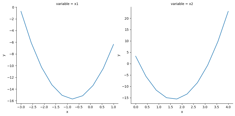
# Obtain plots without vertical x lines
pjp.proj_plot(obj_fun, x_opt=x_opt, x_lims=x_lims,
              x_names=x_names, n_pts=n_pts)

<seaborn.axisgrid.FacetGrid at 0x7f5f6f40ae90>

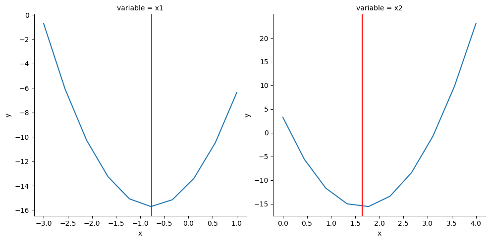
# Obtain plots with vertical x lines
pjp.proj_plot(obj_fun, x_opt=x_opt, x_lims=x_lims,
              x_names=x_names, n_pts=n_pts,
              opt_vlines=True)

<seaborn.axisgrid.FacetGrid at 0x7f5f6f688690>

Advanced Use Cases

In these cases, the calculation of the x-value matrix, projection DataFrame and plotting are done separately. Another added feature is that the user is able to plot vertical lines on the projection plots by providing an array whereas with projplot.proj_plot() this can only be done at the optimal values.

# Generate first round of x_values
x_vals = pjp.proj_xvals(x_opt, x_lims, n_pts)
x_vals

array([[-3.        ,  1.647     ],
       [-2.55555556,  1.647     ],
       [-2.11111111,  1.647     ],
       [-1.66666667,  1.647     ],
       [-1.22222222,  1.647     ],
       [-0.77777778,  1.647     ],
       [-0.33333333,  1.647     ],
       [ 0.11111111,  1.647     ],
       [ 0.55555556,  1.647     ],
       [ 1.        ,  1.647     ],
       [-0.765     ,  0.        ],
       [-0.765     ,  0.44444444],
       [-0.765     ,  0.88888889],
       [-0.765     ,  1.33333333],
       [-0.765     ,  1.77777778],
       [-0.765     ,  2.22222222],
       [-0.765     ,  2.66666667],
       [-0.765     ,  3.11111111],
       [-0.765     ,  3.55555556],
       [-0.765     ,  4.        ]])

# Obtain a DataFrame for plotting
plot_data = pjp.proj_data(obj_fun, x_vals, x_names)
plot_data

	y	x	variable
0	-0.715737	-3.000000	x1
1	-6.084033	-2.555556	x1
2	-10.267144	-2.111111	x1
3	-13.265070	-1.666667	x1
4	-15.077811	-1.222222	x1
5	-15.705367	-0.777778	x1
6	-15.147737	-0.333333	x1
7	-13.404922	0.111111	x1
8	-10.476922	0.555556	x1
9	-6.363737	1.000000	x1
10	3.285675	0.000000	x2
11	-5.580498	0.444444	x2
12	-11.681239	0.888889	x2
13	-15.016547	1.333333	x2
14	-15.586424	1.777778	x2
15	-13.390868	2.222222	x2
16	-8.429881	2.666667	x2
17	-0.703461	3.111111	x2
18	9.788391	3.555556	x2
19	23.045675	4.000000	x2

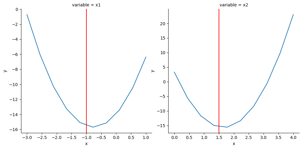
# Plot vertical line at value specified by vlines
vlines = np.array([-1., 1.5]) # different from x_opt
pjp.proj_plot_show(plot_data, vlines=vlines)

<seaborn.axisgrid.FacetGrid at 0x7f5f737efe90>

Vectorized Function

In the above, obj_fun() can only take a single vector x at a time. Inside projplot.proj_plot() (or projplot.proj_data()) the function is run through a for-loop on each value of x. Alternatively, obj_fun() can be vectorized over each row of x by providing the projplot functions with the argument vectorized=True.

def obj_fun_vec(x):
    '''
    Vectorized computation of x'Ax - 2b'x.

    Params: 
        x: A nx2 vector.

    Returns:
        The output of x'Ax - 2b'x applied to each row of x.
    '''
    x = x.T
    y = np.diag(x.T.dot(A).dot(x)) - 2 * b.dot(x)
    return y


pjp.proj_plot(obj_fun_vec, x_opt=x_opt, x_lims=x_lims,
              x_names=x_names, n_pts=n_pts,
              vectorized=True,
              opt_vlines=True)

<seaborn.axisgrid.FacetGrid at 0x7f5f6c5a1810>

We can see that the produced plots for the vectorized and non-vectorized function are identical. Vectorized functions have the advantage of running more efficiently; however, they are not necessary to utilize projplot.